crispyx tutorial

Genome-wide CRISPR screens routinely produce datasets with hundreds of thousands of cells and tens of thousands of genes. Standard single-cell toolkits (Scanpy, Pertpy) load the entire count matrix into memory, which can require 30–100+ GB of RAM. crispyx streams data directly from on-disk AnnData .h5ad files so that QC, normalisation, pseudo-bulk aggregation, and differential expression all run without materialising the full matrix. These memory savings assume sufficient free disk space for streaming intermediates and output files — crispyx warns automatically if that looks tight, and cx.estimate_disk_usage(...) can check usage before a large run (see the Disk space section of Working with large data).

This tutorial walks through a complete crispyx workflow on the included Adamson subset dataset, covering:

1. Data loading and inspection

2. Data preparation utilities

3. Quality control

4. Subsampling and downsampling

5. Streaming normalisation

6. Dimension reduction (PCA, KNN, UMAP)

7. Pseudo-bulk aggregation

8. Differential expression (Wilcoxon and NB-GLM)

9. LFC shrinkage

10. Plotting

For the full API, see the API reference; each step’s guide page is linked from the Quick start.

Setup

Install the project in editable mode (with the optional test extras) to make the package importable:

pip install -e .[test]

1. Load the dataset

This tutorial uses the included Adamson subset stored at data/Adamson_subset.h5ad. cx.read_h5ad_ondisk returns a read-only wrapper — the expression matrix stays on disk.

import sys
from pathlib import Path
import pandas as pd

# Paths stay relative to this notebook's directory so that the paths crispyx
# echoes in its output are the same on every machine.
ROOT = Path('../..')
sys.path.insert(0, str(ROOT))
sys.path.insert(0, str(ROOT / 'src'))
DATA_PATH = ROOT / 'data' / 'Adamson_subset.h5ad'
OUTPUT_DIR = Path('tutorial_outputs')
OUTPUT_DIR.mkdir(parents=True, exist_ok=True)

import crispyx as cx
print(f'crispyx {cx.__version__}')

if not DATA_PATH.exists():
    raise FileNotFoundError(f'Expected dataset at {DATA_PATH}')

crispyx 0.2.0

Inspect metadata

The obs and var accessors expose head and load helpers so you can preview metadata without materialising the entire object.

adata_ro = cx.read_h5ad_ondisk(DATA_PATH)
adata_ro

AnnData object with n_obs × n_vars = 1716 × 11630 backed at '../../data/Adamson_subset.h5ad'
    obs: 'perturbation', 'n_genes', 'dataset', 'celltype'
    var: 'Ensembl_ID'
First obs rows:
                 perturbation  n_genes  dataset celltype
Cell_barcodes
AAACATACAAGATG-1      control     2914  Adamson     K562
AAACATTGCATTGG-1      control     3999  Adamson     K562
AAACGGCTAATGCC-1       AMIGO3     3947  Adamson     K562
AAAGACGAACTCAG-1      control     2713  Adamson     K562
AAAGAGACTCGCCT-1      control     3678  Adamson     K562
First var rows:
                  Ensembl_ID
Gene_symbol
LINC00115    ENSG00000225880
NOC2L        ENSG00000188976
KLHL17       ENSG00000187961
HES4         ENSG00000188290
ISG15        ENSG00000187608

AnnData(path=../../data/Adamson_subset.h5ad, mode='r')

adata_ro.obs.head()

	perturbation	n_genes	dataset	celltype
Cell_barcodes
AAACATACAAGATG-1	control	2914	Adamson	K562
AAACATTGCATTGG-1	control	3999	Adamson	K562
AAACGGCTAATGCC-1	AMIGO3	3947	Adamson	K562
AAAGACGAACTCAG-1	control	2713	Adamson	K562
AAAGAGACTCGCCT-1	control	3678	Adamson	K562

adata_ro.var.head()

	Ensembl_ID
Gene_symbol
LINC00115	ENSG00000225880
NOC2L	ENSG00000188976
KLHL17	ENSG00000187961
HES4	ENSG00000188290
ISG15	ENSG00000187608

2. Data preparation utilities

crispyx provides helpers to inspect and standardise metadata in backed h5ad files without loading the expression matrix.

# Feature 1: load obs/var without reading X
obs = cx.load_obs(DATA_PATH)
print('obs columns:', list(obs.columns))
print('obs shape:  ', obs.shape)

var = cx.load_var(DATA_PATH)
print('var columns:', list(var.columns))
print('var shape:  ', var.shape)

obs columns: ['perturbation', 'n_genes', 'dataset', 'celltype']
obs shape:   (1716, 4)
var columns: ['Ensembl_ID']
var shape:   (11630, 1)

# Feature 4: auto-detect perturbation and gene columns
cols = cx.infer_columns(DATA_PATH)
print('Detected columns:', cols)

[cx] detect_perturbation_column: Detected 'perturbation' (score=8)
Detected columns: {'perturbation_column': 'perturbation', 'gene_name_column': None}

# Feature 3: normalise perturbation labels (inplace=False for preview)
normalised = cx.normalise_perturbation_labels(
    DATA_PATH,
    column='perturbation',
    canonical_control='NTC',
    inplace=False,
)
print(normalised.value_counts().head(10))

perturbation
AMIGO3    750
NTC       500
AARS      466
Name: count, dtype: int64

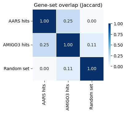
# Feature 5: overlap analysis between gene sets from different perturbations
# (Using toy sets for illustration; in practice, fill with DE-significant genes)
de_sets = {
    'AARS hits':  {'ATF4', 'DDIT3', 'ASNS', 'EIF2AK4', 'SLC7A5'},
    'AMIGO3 hits': {'ATF4', 'DDIT3', 'CDK4', 'CDKN1A', 'EGFR'},
    'Random set': {'BRCA1', 'TP53', 'KRAS', 'EGFR', 'MYC'},
}

result = cx.tl.compute_overlap(de_sets)
print('Jaccard matrix:')
print(result.jaccard_matrix.round(3))
print('\nSet sizes:', result.set_sizes.to_dict())

ax = cx.pl.overlap_heatmap(result, metric='jaccard', title='Gene-set overlap (Jaccard)')

Jaccard matrix:
             AARS hits  AMIGO3 hits  Random set
AARS hits         1.00        0.250       0.000
AMIGO3 hits       0.25        1.000       0.111
Random set        0.00        0.111       1.000

Set sizes: {'AARS hits': 5, 'AMIGO3 hits': 5, 'Random set': 5}

3. Quality control

The cx.pp preprocessing namespace mirrors Scanpy’s API. Each function returns a new cx.AnnData object backed by an .h5ad file on disk.

qc_result = cx.quality_control_summary(
    adata_ro,
    perturbation_column='perturbation',
    min_genes=5,
    min_cells_per_perturbation=5,
    output_dir=OUTPUT_DIR,
    data_name='tutorial',
)
qc_preview = pd.DataFrame(
    {
        'perturbation': adata_ro.obs['perturbation'],
        'qc_pass': qc_result.cell_mask,
    }
)
adata_ro = qc_result.filtered
print(f"QC result: {qc_result.cell_mask.sum()} / {len(qc_result.cell_mask)} cells passed")
qc_preview.head(5)

[cx] pp.qc_summary: Reading ../../data/Adamson_subset.h5ad
[cx] resolve_control_label: Inferred control label 'control'
[cx] pp.qc_summary: Saving → tutorial_outputs/tutorial_cx_filtered.h5ad
[cx] pp.qc_summary: Strategy — in-memory (0.1 GB, estimated 0.2 GB in memory)
[cx] pp.qc_summary: Done  1716/1716 cells kept (100%), 9238/11630 genes kept (79%), 3/3 perturbations kept (100%)
QC result: 1716 / 1716 cells passed

	perturbation	qc_pass
Cell_barcodes
AAACATACAAGATG-1	control	True
AAACATTGCATTGG-1	control	True
AAACGGCTAATGCC-1	AMIGO3	True
AAAGACGAACTCAG-1	control	True
AAAGAGACTCGCCT-1	control	True

Aggressive-filtering warning

crispyx warns when a filtering step drops more than half the data – often a sign of a misconfigured threshold. The Adamson subset above passes QC cleanly, so here is a deliberately strict min_genes cutoff on the same data to show what that warning looks like:

# Deliberately strict threshold to demonstrate the aggressive-filtering warning.
# Captured and printed rather than let through, so the recorded output shows the
# warning itself instead of this machine's path to qc.py.
import warnings

with warnings.catch_warnings(record=True) as caught:
    warnings.simplefilter('always')
    _ = cx.pp.filter_cells(adata_ro, min_genes=4200)

for warning in caught:
    print(f'{warning.category.__name__}: {warning.message}')

[cx] pp.filter_cells: Done  330/1716 cells kept (19%)
UserWarning: pp.filter_cells: only 330/1716 cells (19%) passed filtering. Check your thresholds if this is unexpected.

4. Subsampling and downsampling

Datasets are sometimes larger than a particular analysis needs, or imbalanced across perturbations/batches in ways that confound comparisons (for example, a screen with many more cells per perturbation, or much greater sequencing depth per cell, than the dataset you want to compare it against). cx.pp.subsample and cx.pp.downsample_counts reduce scale along two different, composable axes, both streaming and without materialising the full matrix:

• ``cx.pp.subsample`` decides which cells survive. Stratify by one or more obs columns with groupby, and draw either an exact count (n) or a proportion (frac) independently within each stratum. unit="cell" (default) draws individual cells; passing an obs column name instead (e.g. unit="batch") switches to cluster sampling — a chosen unit’s cells are kept in full and an unchosen unit’s cells are dropped in full, useful when a dataset has many batches and the goal is to reduce how many batches are processed, not just how many cells within them. drop_insufficient controls what happens to a stratum smaller than the requested count: drop it entirely (default), or keep it in full.

• ``cx.pp.downsample_counts`` decides how many counts survive within a surviving cell — it thins each cell’s total UMI/read count down to a target via sampling without replacement (the same distribution scanpy.pp.downsample_counts(..., replace=False) produces, computed natively so this stays a crispyx-only dependency), useful for equalising sequencing depth before comparing cells or datasets.

Both operate on .obs metadata or raw counts respectively, so run them before normalisation.

# Stratified subsample: cap every perturbation group at n=200 cells each
# (a group smaller than that would be kept in full since drop_insufficient=False).
# Written to a separate file -- adata_ro itself is untouched, so the rest of
# this tutorial keeps using the full QC-filtered dataset.
adata_sub = cx.pp.subsample(
    adata_ro,
    n=200,
    groupby='perturbation',
    drop_insufficient=False,
    random_state=0,
    data_name='tutorial_subsample',
)
print(f"Subsampled shape: {adata_sub.shape}")
adata_sub.obs.load()['perturbation'].value_counts()

[cx] pp.subsample: Done  600/1716 cells kept (35%) across 3 stratum/strata (unit='cell')
Subsampled shape: (600, 9238)

perturbation
AARS       200
AMIGO3     200
control    200
Name: count, dtype: int64

# Downsample counts: thin every cell's total UMI count down to a target,
# leaving cells already at or below the target unchanged. Runs on raw counts
# (adata_ro is still pre-normalisation here), so this is the right point in
# the pipeline for it -- do it before cx.pp.normalize_total_log1p, not after.
import numpy as np

lib_sizes = np.asarray(adata_ro.to_memory().X.sum(axis=1)).ravel()
target = int(np.median(lib_sizes))
print(f"Library size before: median={np.median(lib_sizes):.0f}, max={lib_sizes.max():.0f}")

adata_ds = cx.pp.downsample_counts(
    adata_ro,
    counts_per_cell=target,
    random_state=0,
    data_name='tutorial_downsample',
)
lib_after = np.asarray(adata_ds.to_memory().X.sum(axis=1)).ravel()
print(f"Library size after:  median={np.median(lib_after):.0f}, max={lib_after.max():.0f}")

Library size before: median=14508, max=44938
[cx] pp.downsample_counts: Saving → tutorial_outputs/tutorial_downsample_cx_downsample_counts.h5ad

pp.downsample_counts: 100%|██████████| 1/1 [00:00<00:00,  2.24chunk/s]

[cx] pp.downsample_counts: Done  858/1716 cells thinned to <= 14508 counts
Library size after:  median=14505, max=14508

5. Streaming normalisation

For large datasets that would OOM during normalisation, use the streaming preprocessing function. This is the equivalent of scanpy.pp.normalize_total() + scanpy.pp.log1p() but processes data in chunks.

# Create a normalized + log1p version of the QC-filtered data (streaming)
# This works on huge datasets without loading into memory
adata_norm = cx.pp.normalize_total_log1p(
    adata_ro,  # Pass the AnnData object directly (same as other cx.pp functions)
    output_dir=OUTPUT_DIR,
    data_name='tutorial',
    target_sum=1e4,  # Same as scanpy default
    verbose=True,
)

# Verify the output - adata_norm is a read-only AnnData wrapper
print(f"Shape: {adata_norm.shape}")
print(f"First 3 cells, first 3 genes:\n{adata_norm.to_memory().X[:3, :3].toarray()}")

[cx] pp.normalize_total_log1p: Saving → tutorial_outputs/tutorial_cx_normalized_log1p.h5ad
[cx] pp.normalize_total_log1p: Done  1716 cells × 9238 genes
Shape: (1716, 9238)
First 3 cells, first 3 genes:
[[0.75838053 0.         0.        ]
 [0.49522132 0.         0.        ]
 [1.4766263  0.         0.5161892 ]]

6. Dimension reduction

crispyx provides streaming PCA and KNN graph construction that works on backed (on-disk) AnnData objects.

• Streaming PCA: Automatically selects the optimal method based on gene count (sparse_cov for ≤15K genes, incremental for larger).

• KNN neighbors: Builds k-nearest neighbor graph from PCA embeddings for downstream clustering/UMAP.

Results are written directly to the h5ad file using a close-write-reopen pattern.

# Streaming PCA on the normalized data
# Results are written directly to the h5ad file (close-write-reopen pattern)
cx.pp.pca(adata_norm, n_comps=20, show_progress=True)

# Check PCA results (data is read from the h5ad file)
print(f"PCA embeddings shape: {adata_norm.obsm['X_pca'].shape}")
print(f"Variance explained: {adata_norm.uns['pca']['variance_ratio'][:5]}")  # First 5 components

# Build KNN graph from PCA embeddings (also writes to h5ad)
cx.pp.neighbors(adata_norm, n_neighbors=10, method='sklearn', show_progress=True)

print(f"KNN distances shape: {adata_norm.obsp['distances'].shape}")
print(f"Number of connections: {adata_norm.obsp['connectivities'].nnz}")

PCA embeddings shape: (1716, 20)
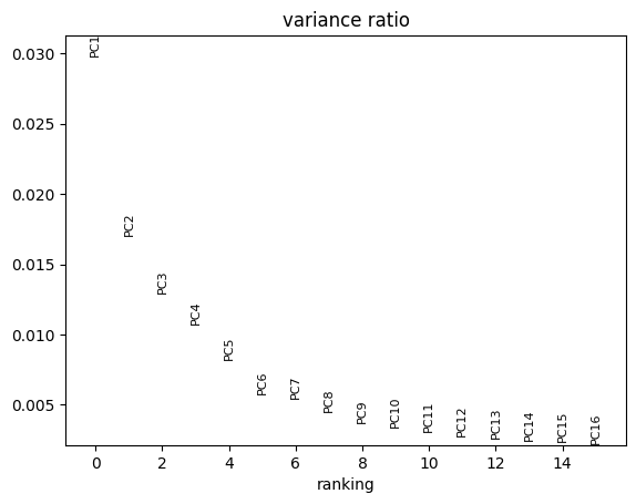
Variance explained: [0.02978331 0.01700597 0.01289528 0.01072035 0.00821617]
KNN distances shape: (1716, 1716)
Number of connections: 25228

PCA visualization

The cx.pl namespace provides Scanpy-style plotting wrappers:

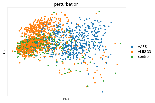
• cx.pl.pca(): Scatter plot of PCA embeddings

• cx.pl.pca_variance_ratio(): Explained variance per component

• cx.pl.pca_loadings(): Gene loadings for top components

# Plot PCA variance explained
cx.pl.pca_variance_ratio(adata_norm, n_pcs=15)

# Plot PCA scatter colored by perturbation
cx.pl.pca(adata_norm, color='perturbation', components='1,2')

# Plot gene loadings for first 3 components
cx.pl.pca_loadings(adata_norm, components=[1, 2, 3])

UMAP visualization

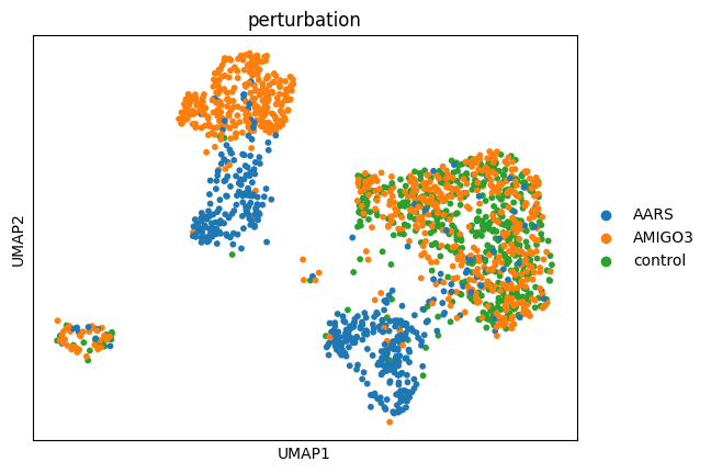
After computing PCA and building the neighbor graph, we can compute UMAP embeddings for visualization. cx.tl.umap() uses the pre-computed neighbor graph from cx.pp.neighbors(), so it only loads the neighbor matrix (not the full expression matrix) into memory.

This is memory-efficient: approximately 0.75 MB per 1000 cells for 15 neighbors.

# Compute UMAP from neighbor graph (memory-efficient)
cx.tl.umap(adata_norm, min_dist=0.5, spread=1.0)

# Check UMAP results
print(f"UMAP embedding shape: {adata_norm.obsm['X_umap'].shape}")

# Plot UMAP colored by perturbation
cx.pl.umap(adata_norm, color='perturbation')

WARNING: .obsp["connectivities"] have not been computed using umap
UMAP embedding shape: (1716, 2)

7. Pseudo-bulk with cx.pb

cx.pb separates two different jobs:

• ``cx.pb.aggregate`` returns an absolute profile per group. No reference is involved. Include batch in groupby to keep one profile per perturbation and batch, which gives replicate-aware input for downstream models.

• ``cx.pb.normalized_effects`` returns a contrast against a reference, library-size normalised, in one streaming pass. Pass batch_column= on multi-batch data to compute the effect within each batch and combine with harmonic weights.

• ``cx.pb.effects`` is the same contrast but on whatever scale its input already carries, and it accepts a saved cx.pb.aggregate artifact so profiles can be reused without re-reading the cell matrix.

This dataset has no batch column, so the calls below are the single-batch case.

cx.pb.aggregate needs an explicit method: 'sum' gives the raw-count sums that count models (DESeq2, nb_glm_test) need, 'mean_log1p' the mean of log1p values for log-scale contrasts. Each profile is named by its group key (values joined with | for several groupby columns), and obs keeps every input column that is constant within a profile – donor covariates, for instance – next to the cell counts n_cells.

profiles = cx.pb.aggregate(
    adata_ro,
    groupby='perturbation',
    method='mean_log1p',  # required: 'sum' for count models, 'mean_log1p' for log-scale contrasts
    output_dir=OUTPUT_DIR,
    data_name='tutorial',
)
print(f"Absolute profiles: {profiles.shape}")
# Rows are named by their group; obs columns constant within each profile
# (dataset, celltype) are carried over, per-cell ones (n_genes) are not.
profiles.obs.head()

[cx] pb.aggregate: chunk_size=4096 (auto)
[cx] pb.aggregate: detected count data; applying log1p before averaging
[cx] pb.aggregate accumulator: estimated disk usage: 221.7 KB (151.7 GB free)
[cx] pb.aggregate: estimated disk usage: 243.9 KB (151.7 GB free)

pb.aggregate: 100%|██████████| 1/1 [00:00<00:00,  8.43chunk/s]

[cx] pb.aggregate: obs columns that vary within a profile are not carried over: ['n_genes']
[cx] pb.aggregate: 3 profiles × 9238 genes
[cx] pb.aggregate: Saving → tutorial_outputs/tutorial_cx_pseudobulk_mean_log1p.h5ad
Absolute profiles: (3, 9238)

	perturbation	dataset	celltype	n_cells	n_cells_aggregated	sampled_with_replacement
pseudobulk_id
control	control	Adamson	K562	500	500	False
AMIGO3	AMIGO3	Adamson	K562	750	750	False
AARS	AARS	Adamson	K562	466	466	False

# Contrast against the control, normalised internally.
# On multi-batch data add batch_column='batch' for the batch-corrected effect.
effects = cx.pb.normalized_effects(
    adata_ro,
    groupby='perturbation',
    method='mean_log1p',
    output_dir=OUTPUT_DIR,
    data_name='tutorial',
)
print(f"Effects: {effects.shape}  layers: {list(effects.backed.layers)}")
effects.obs.head()

[cx] pb.normalized_effects: Reading tutorial_outputs/tutorial_cx_filtered.h5ad
[cx] pb.normalized_effects: chunk_size=4096 (auto)
[cx] resolve_control_label: Inferred control label 'control'
[cx] pb.normalized_effects: estimated disk usage: 650.4 KB (151.7 GB free)
[cx] pb.normalized_effects: 2 perturbations × 9238 genes
[cx] pb.normalized_effects: Saving → tutorial_outputs/tutorial_cx_normalized_effects.h5ad
Effects: (2, 9238)  layers: ['perturbation_profile', 'standard_error', 'standard_error_robust']

	perturbation
perturbation
AMIGO3	AMIGO3
AARS	AARS

8. Differential expression with cx.tl

Run a Wilcoxon test that mirrors scanpy.tl.rank_genes_groups. cx.AnnData.uns entries also provide preview and load helpers.

Checking disk usage before a large run

Before running an expensive test, cx.estimate_disk_usage (also available as cx.tl.estimate_disk_usage) reports how much disk space it will need without touching the expression matrix – useful for capacity planning before committing to a run on a shared cluster. On this small tutorial subset the footprint is negligible, but the same call on a genome-wide screen reports a meaningful number.

usage = cx.tl.estimate_disk_usage(
    'wilcoxon_test',
    adata_norm.path,
    perturbation_column='perturbation',
)
for location, estimate in usage.items():
    print(f'{location}: {estimate}')

[cx] resolve_control_label: Inferred control label 'control'
output: 1.9 MB required, 151.7 GB free at tutorial_outputs [OK]

adata_ro = cx.tl.rank_genes_groups(
    adata_norm,  # Wilcoxon expects log-normalized data
    perturbation_column='perturbation',
    method='wilcoxon',
    output_dir=OUTPUT_DIR,
    data_name='tutorial',
)

# Preview a tidy DE table using plotting helper (no scanpy_format needed)
group = adata_ro.obs.load()['perturbation'].astype(str).unique()[0]
cx.pl.rank_genes_groups_df(adata_ro, group=group, n_genes=10).head()

[cx] resolve_control_label: Inferred control label 'control'
[cx] wilcoxon_test: chunk_size=4096 (auto)
[cx] wilcoxon_test: format_mismatch_policy='auto': streaming from the source (3 chunks x 48.3 MB at 6.7 GB/s = 0.01 s per re-read, 0.0 s of re-reading beyond the first chunk)
[cx] wilcoxon_test: Strategy — single-pass
[cx] wilcoxon_test: estimated disk usage: 1.9 MB (151.7 GB free)

Wilcoxon DE (gene chunks): 100%|██████████| 3/3 [00:00<00:00,  4.99perturbation/s]

[cx] Wilcoxon DE: 2 perturbations complete, mean 9238/9238 genes tested (100%)
[cx] wilcoxon_test: Saving → tutorial_outputs/tutorial_cx_wilcoxon.h5ad

	names	scores	logfoldchanges	pvals	pvals_adj	pts	pts_rest	group
0	SET	-10.899647	-0.506634	1.157049e-27	8.419143e-24	0.990667	0.988	AMIGO3
1	MT-CO2	10.858218	0.402062	1.822720e-27	8.419143e-24	0.998667	0.998	AMIGO3
2	RPS27A	10.551140	0.267033	5.018421e-26	1.022991e-22	1.000000	1.000	AMIGO3
3	EIF1	10.539785	0.288907	5.662821e-26	1.022991e-22	1.000000	1.000	AMIGO3
4	MT-CYB	10.534347	0.327073	5.999814e-26	1.022991e-22	0.998667	0.998	AMIGO3

Use load to materialise the complete differential expression tables for downstream analysis.

group = adata_ro.obs.load()['perturbation'].astype(str).unique()[0]
top_df = cx.pl.rank_genes_groups_df(adata_ro, group=group, n_genes=5)
print(f"Top 5 DE genes for perturbation '{group}':")
top_df[['names', 'logfoldchanges', 'pvals_adj']]

Top 5 DE genes for perturbation 'AMIGO3':

	names	logfoldchanges	pvals_adj
0	SET	-0.506634	8.419143e-24
1	MT-CO2	0.402062	8.419143e-24
2	RPS27A	0.267033	1.022991e-22
3	EIF1	0.288907	1.022991e-22
4	MT-CYB	0.327073	1.022991e-22

The cx.AnnData handles close themselves when their Python objects go out of scope, so no explicit cleanup is required.

9. NB-GLM differential expression

For more sophisticated differential expression analysis, crispyx provides a negative binomial GLM method that models count data directly. This is especially useful when you need to incorporate covariates or want more accurate statistical modeling.

Note: NB-GLM operates on raw counts (not log-normalized data), so we use the QC-filtered dataset directly.

# Run NB-GLM test on raw counts
# First, reload the QC-filtered dataset (not log-normalized)
qc_path = OUTPUT_DIR / 'tutorial_cx_filtered.h5ad'
adata_qc = cx.read_h5ad_ondisk(qc_path)

adata_nb = cx.tl.rank_genes_groups(
    adata_qc,
    perturbation_column='perturbation',
    method='nb_glm',
    output_dir=OUTPUT_DIR,
    data_name='tutorial_nb',
)
group = adata_nb.obs.load()['perturbation'].astype(str).unique()[0]
cx.pl.rank_genes_groups_df(adata_nb, group=group, n_genes=5).head()

AnnData object with n_obs × n_vars = 1716 × 9238 backed at 'tutorial_outputs/tutorial_cx_filtered.h5ad'
    obs: 'perturbation', 'n_genes', 'dataset', 'celltype'
    var: 'Ensembl_ID', 'gene_symbols'
First obs rows:
                 perturbation  n_genes  dataset celltype
Cell_barcodes
AAACATACAAGATG-1      control     2914  Adamson     K562
AAACATTGCATTGG-1      control     3999  Adamson     K562
AAACGGCTAATGCC-1       AMIGO3     3947  Adamson     K562
AAAGACGAACTCAG-1      control     2713  Adamson     K562
AAAGAGACTCGCCT-1      control     3678  Adamson     K562
First var rows:
                  Ensembl_ID gene_symbols
Gene_symbol
NOC2L        ENSG00000188976        NOC2L
KLHL17       ENSG00000187961       KLHL17
HES4         ENSG00000188290         HES4
ISG15        ENSG00000187608        ISG15
AGRN         ENSG00000188157         AGRN
[cx] resolve_control_label: Inferred control label 'control'
[cx] nb_glm_test: chunk_size=256 (auto)
[cx] nb_glm_test: estimated disk usage: 3.5 MB (151.7 GB free)

NB-GLM DE: 100%|██████████| 2/2 [00:01<00:00,  1.14perturbation/s]

[cx] NB-GLM DE: 2/2 perturbations complete, mean 9238/9238 genes tested (100%)
[cx] nb_glm_test: Saving → tutorial_outputs/tutorial_nb_cx_nb_glm.h5ad

	names	scores	logfoldchanges	pvals	pvals_adj	pts	pts_rest	group
0	MT-CO2	10.750632	0.447593	5.885681e-27	5.437192e-23	0.998667	0.998	AMIGO3
1	HIST1H1E	-10.153440	-0.832827	3.198863e-24	1.477555e-20	0.512000	0.738	AMIGO3
2	MT-CYB	10.048626	0.402681	9.315763e-24	2.868634e-20	0.998667	0.998	AMIGO3
3	UQCRB	9.467183	0.538119	2.874926e-21	5.305221e-18	0.952000	0.918	AMIGO3
4	EIF1	9.455920	0.356261	3.201925e-21	5.305221e-18	1.000000	1.000	AMIGO3

10. LFC shrinkage with apeGLM

Apply adaptive shrinkage to log-fold changes using the apeGLM method. This shrinks noisy/uncertain LFCs toward zero while preserving large effects, following DESeq2/PyDESeq2 best practices.

The two-step workflow (NB-GLM → shrink_lfc) gives you control over when shrinkage is applied and allows you to compare shrunk vs unshrunk results.

# Apply LFC shrinkage to NB-GLM results
nb_result_path = adata_nb.path

shrunk = cx.tl.shrink_lfc(
    nb_result_path,
    prior_scale_mode='global',  # Use global prior across all perturbations
)

# Compare shrunk vs raw LFC for a perturbation
import anndata
shrunk_adata = anndata.read_h5ad(shrunk.result_path)
print("Shrunk vs Raw LFC (first 5 genes, first perturbation):")
print(f"  Shrunk LFC: {shrunk_adata.X[0, :5]}")
print(f"  Raw LFC:    {shrunk_adata.layers['logfoldchange_raw'][0, :5]}")

[cx] shrink_lfc: estimated disk usage: 2.0 MB (151.7 GB free)
[cx] shrink_lfc: Saving → tutorial_outputs/tutorial_nb_cx_nb_glm_shrunk.h5ad
[cx] shrink_lfc: Done  2 perturbations × 9238 genes (method='stats')
Shrunk vs Raw LFC (first 5 genes, first perturbation):
  Shrunk LFC: [ 0.00049389 -0.01187052  0.01916586  0.03188859 -0.04617658]
  Raw LFC:    [ 0.00056502 -0.02613842  0.02466158  0.03882457 -0.07999897]

The shrunk LFC values are typically smaller in magnitude for genes with high uncertainty, while large, well-supported effects are preserved. This improves downstream ranking and visualization.

11. Plotting (Scanpy-style)

crispyx provides cx.pl helpers for plotting on-disk results. The examples below mirror Scanpy style while keeping the expression matrix on disk.

# QC plots
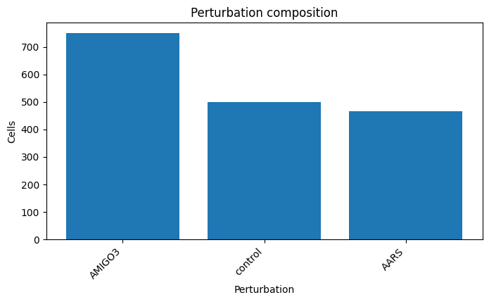
cx.pl.qc_perturbation_counts(
    data=adata_qc,
    perturbation_column='perturbation',
    cell_mask=qc_result.cell_mask,
)
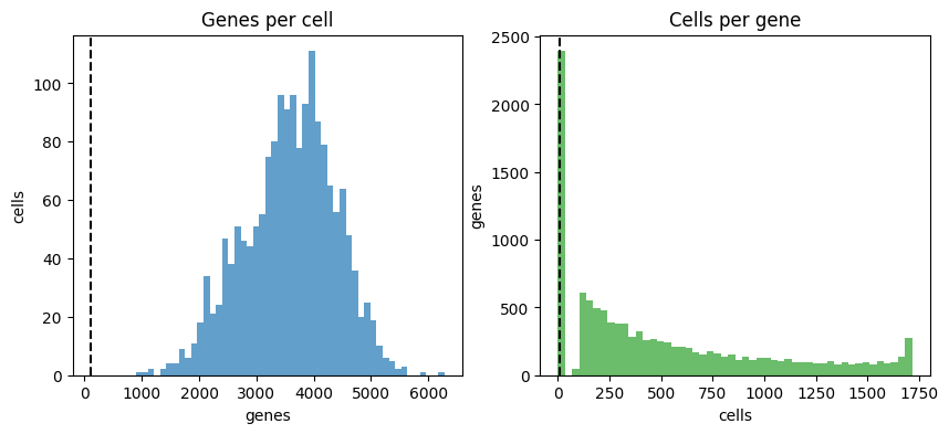
cx.pl.qc_summary(qc_result, min_genes=100, min_cells_per_gene=10)

# Rank genes groups plot
cx.pl.rank_genes_groups(adata_ro, n_genes=20, sharey=False)

# Volcano / top genes
plot_group = adata_ro.obs.load()['perturbation'].astype(str).unique()[0]
df = cx.pl.rank_genes_groups_df(adata_ro, group=plot_group, n_genes=200)
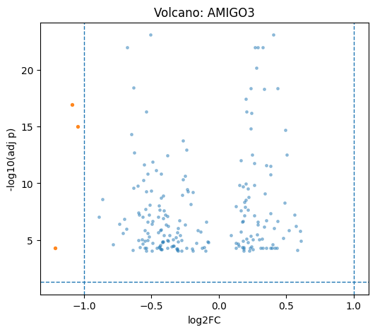
cx.pl.volcano(de_df=df, group=plot_group)
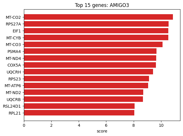
cx.pl.top_genes_bar(de_df=df, group=plot_group, topn=15)

# MA plot (raw counts from QC-filtered data)
try:
    control_label = adata_ro.uns['control_label'].load()
except KeyError:
    control_label = 'control'
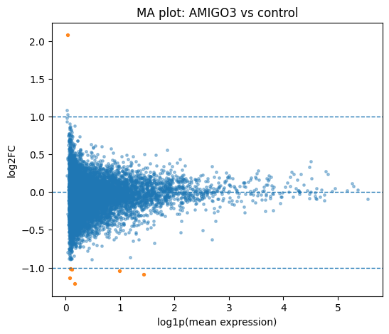
cx.pl.ma(
    data=adata_qc,
    de_result=adata_ro,
    group=plot_group,
    reference=control_label,
    perturbation_column='perturbation',
    mean_mode='raw',
)

<Axes: title={'center': 'MA plot: AMIGO3 vs control'}, xlabel='log1p(mean expression)', ylabel='log2FC'>